The US Long-Short Portfolio: Tail-Weighted Forecasts and Sensitivity to Delisting Assumptions

The US Long-Short Portfolio is a monthly, dollar-neutral book built on 147 characteristics from Jensen, Kelly, and Pedersen (2023) across 529,082 US stock-months. In an event-driven simulation from $10 million over January 2021 to August 2026, it has a net information ratio of 3.77 against T-bill + 4%, 12.4% volatility, and 18.19× growth.

Those figures should not be read as achievable returns. The design passed through 65 trials that had seen the evaluation window, about 91% of short gross sits in micro- and nano-capitalisation stocks, and borrow availability is modelled and not observed. The paper (PDF) has the full method, tables, and references.

Forecast and alpha

Each January, a Ridge regression and a tail-weighted XGBoost model are refit on all earlier months, and their cross-sectional $z$-scores are averaged. The 200 highest and 200 lowest scores among tradable names become candidates. Alpha then follows the fundamental law of Grinold and Kahn (2000), with a confidence weight from conformalised quantile regression:

$$\alpha_{i,t} = \mathrm{IC}^+_{\text{leg}(i),t}\,\sigma_{i,t}\,z_{i,t}\,\mathrm{conf}_{i,t},$$

where $\mathrm{IC}^+_{\text{leg},t}$ is the leg’s rank IC over the last 36 months, floored at zero.

Skill sits on the short side

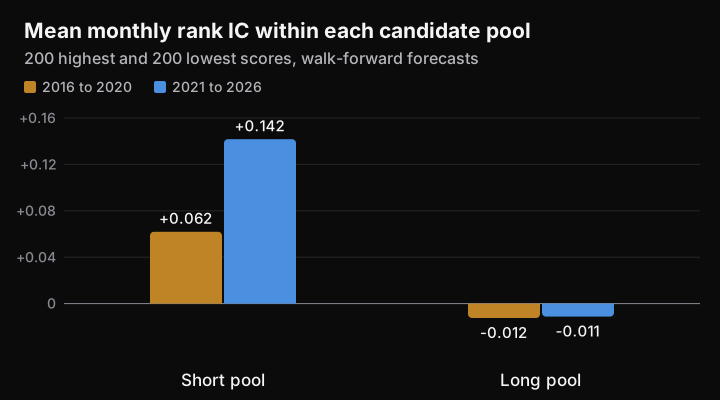
The chart above shows the book’s defining asymmetry. Rank IC is strongly positive in the short pool and slightly negative in the long pool, so the long floor binds in 82% of months before 2021 and 91% after. In the evaluation window, shorts contribute +44.8% a year and longs +9.8%, and longs mostly hedge the factor, beta, and industry exposure of the shorts.

The skill also appears in the median stock and not the mean. The bottom quintile by score has a median return about 1.3 to 1.4% a month below the universe ($t = -3.5$), but its mean difference is zero ($t = 0.0$). Forecasts find typical losers, and rare large winners in the same names offset them. QUARCC Purple, which keeps a $500 million floor on shorts, works in the same anomaly territory without access to those names.

Risk and construction

The covariance adds an alpha-alignment factor (Ceria, Saxena, and Stubbs, 2012) and a diagonal adverse-tail term built from the 0.99 conformal quantile of squeeze risk on shorts and crash risk on longs:

$$\boldsymbol{\Sigma}_t = g_t\big(\boldsymbol{\Sigma}_{F,t} + \sigma_{\text{AAF},t}^2 \hat{\boldsymbol{\alpha}}_t \hat{\boldsymbol{\alpha}}_t^\top\big) + \mathrm{diag}(\mathbf{h}_{\text{tail},t}).$$

A single convex program maximises alpha net of risk, spread, commission, impact, borrow, recall, and a turnover penalty. Long and short legs are each 50% of NAV, beta is limited to ±0.05, the book may not be short market convexity, industry net is limited to ±5%, and single names are capped at 2.5%.

Results

Metric	Portfolio	S&P 500
Growth of $1	18.19	2.05
CAGR	66.8%	13.5%
Volatility	12.36%	15.10%
Sharpe ratio	4.10	0.70
Maximum drawdown	−4.49%	−24.8%
Information ratio vs. T-bill + 4%	3.77	0.44
Beta to the S&P 500	+0.09	1.00
Costs per year	5.2%

All figures are simulated from $10 million, net of modelled costs. Rolling 12-month beta ranges from −0.31 to +0.99, so the low full-sample beta hides real market exposure at times.

Sensitivity to data handling

Three data-handling choices materially affect the results:

1. Look-ahead in the universe. Scoring only stocks with an observed next-month return uses information unavailable at formation. Scoring all stocks restores 2,311 name-months.
2. Exit liquidity. Assigning a delisted name the smallest volume among requested names can make an exit cost up to 244% of notional.
3. Missing returns. One treatment books a held stock with no return at −30% if long and 0 if short. The baseline closes both at the last available price, a return of zero.

Universe and exits	Missing return	IR	Growth	Costs/yr
Original, original exits	−30% long	3.631	17.81	5.13%
All rows, original exits (not kept)	−30% long	3.444	16.27	6.91%
All rows, repaired exits	−30% long	3.602	17.52	5.11%
All rows, repaired exits	Last price	3.769	18.19	5.18%

Fixing the first two problems at the original −30% assumption lowers the IR, from 3.63 to 3.60. The whole gain to 3.77 comes from the third choice, across 189 delisted positions, 147 of them long. Shumway (1997) shows performance-related delistings lose substantially, while cash mergers close near their last price, so the truth lies in between. We regard 3.60 to 3.77 as the plausible range.

Limitations

• Selection. Models are walk-forward, but 65 trials saw 2021 to 2026 results of earlier versions. The deflated Sharpe ratio is 0.886, below the conventional 0.95, and the data-handling corrections were made with results in view.
• Short-book composition. By gross, 91% of the short book is micro- or nano-cap, 61% trades below $5, and the median short has a $58 million market capitalisation. The model charges 3.4% a year for borrow and recall, but it has no record of actual availability or fee history.
• Capacity. Our paper-fund page presents this book on a $1 billion base through a linear 100× rescale, which is for display. On the development window a related 500-name control already has 34 to 42% of short gross beyond one day of 10% of daily volume at $10 million, and its net return stops rising near 100 to 120% gross. Returns at $1 billion would be far lower.
• Paper marks. The same page marks one 31 August 2026 formation forward with market data, and it does not execute trades.

Alternative specifications

No alternative exceeds the baseline information ratio in the evaluation window, and the three development-window specifications below fall below the control.

Variant	Window	IR	Vol.	Max DD	Outcome
500-name control	Evaluation	3.478	12.4%	−4.6%	500-name limit
Normal-rank score blend	Evaluation	3.555			−2.12% a year vs. control ($t = -1.01$)
Volatility target 8%	Evaluation	3.697	8.7%	−3.5%	−11.1% a year vs. control ($t = -3.58$)
Separated $\mu$, $\Sigma$, cost	Evaluation	2.29	29.8%	−28.8%	48.7× growth with a beta of +0.77
Unified compiler (best)	Development	1.04	7.3%	−6.0%	Below control’s 1.36
Fractional IR maximiser	Development	0.24	12.7%	−12.4%	$z = -2.26$ vs. control
LightGBM mean forecast	Development	0.62	31.6%	−57%	Below control’s 1.36

Three results stand out:

• Volatility targeting moves along the frontier. At matched risk on the development window, the target arm and the control have the same frontier, so a higher Sharpe ratio reflects running smaller.
• Spreading bets loses the edge. Policies linear in rank-normalised characteristics hold few small shorts and lose on the short leg, because the skill here is concentrated.
• Placebo test of a joint risk system. In a preregistered 144-month synthetic test against 16 shuffled-forecast placebos with the same risk, cost, and constraints, it lost 0.865% a month (95% CI −2.43% to +0.70%, $p = 0.283$) and ranked last. Its returns arose from the risk, cost, and constraint structure, not from forecast ordering. It was not evaluated on 2021 to 2026 data.

Read more

• Paper (PDF)
• Paper-fund page
• QUARCC Purple