Fast Portfolio Optimisation: Interior-Point Methods That Keep the Structure

Portfolio research solves the same convex problem thousands of times, across gross targets, risk measures, and formation dates. These problems have structure that general-purpose modelling tools discard. In factor-risk QPs, the covariance is a low-rank term plus a diagonal. In scenario models such as CVaR and drawdown, a small dense block of weights couples to a large sparse block of per-scenario variables.

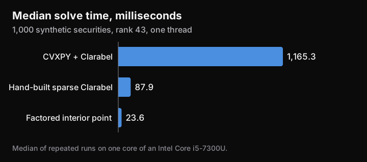
This note describes two interior-point kernels QUARCC built to keep that structure through the solve. A synthetic 1,000-security factor-risk problem takes 23.6 ms in one thread, against 87.9 ms for a hand-built sparse Clarabel model and 1,165.3 ms for CVXPY with Clarabel. At 360,000 scenarios, CVaR models solve 12–17× faster than Riskfolio-Lib. The gain is much smaller on drawdown measures, and some risk-capped problems at that scale fail to converge. The full derivations and every benchmark are in the paper (PDF).

Factor-risk QPs

The first kernel handles a QP in weights $\mathbf{x} \in \mathbb{R}^n$ with box bounds, two-sided exposure bands, and linear equalities:

$$\min_{\mathbf{x}} \; \tfrac{1}{2}\mathbf{x}^\top \mathbf{P}\mathbf{x} + \mathbf{q}^\top \mathbf{x} \quad \text{s.t.} \quad \boldsymbol{\ell} \le \mathbf{x} \le \mathbf{u},\;\; \mathbf{g}_\ell \le \mathbf{G}\mathbf{x} \le \mathbf{g}_u,\;\; \mathbf{A}\mathbf{x} = \mathbf{b}.$$

With factor risk, the Hessian is a low-rank term plus a diagonal, $\mathbf{P} = \mathbf{U}\,\mathrm{diag}(\mathbf{c})\,\mathbf{U}^\top + \mathrm{diag}(\mathbf{p}_d)$. We use a Mehrotra (1992) predictor-corrector. Eliminating slacks leaves a matrix $\mathbf{M} = \mathbf{H} + \mathbf{U}_{\text{aug}}\,\mathrm{diag}(\mathbf{c}_{\text{aug}})\,\mathbf{U}_{\text{aug}}^\top$, where $\mathbf{H}$ is diagonal and each band adds one column. By the Woodbury identity,

$$\mathbf{M}^{-1}\mathbf{V} = \mathbf{H}^{-1}\mathbf{V} - \mathbf{H}^{-1}\mathbf{U}_{\text{aug}}\mathbf{K}^{-1}\mathbf{U}_{\text{aug}}^\top\mathbf{H}^{-1}\mathbf{V}, \qquad \mathbf{K} = \mathrm{diag}(\mathbf{c}_{\text{aug}})^{-1} + \mathbf{U}_{\text{aug}}^\top\mathbf{H}^{-1}\mathbf{U}_{\text{aug}}.$$

Per-iteration linear algebra falls from $O(n^3)$ to $O(nr^2 + r^3)$ for rank $r$. Across a rebalance ladder $\mathbf{U}$, $\mathbf{G}$, and $\mathbf{A}$ do not change, so setup is done once.

Scenario models

The second kernel covers CVaR, worst realisation, mean absolute deviation, semi-deviation, lower partial moments, and drawdown measures, under minimum-risk, utility, maximum-return, and maximum-Sharpe objectives. These share a form with a small dense block $\mathbf{x}$ of size $m$ and a large auxiliary block $\mathbf{v}$:

$$\min_{\mathbf{x},\mathbf{v}} \; \tfrac{1}{2}\mathbf{x}^\top \mathbf{P}\mathbf{x} + \mathbf{c}_x^\top \mathbf{x} + \tfrac{1}{2}\mathbf{v}^\top \mathrm{diag}(\mathbf{q}_v)\mathbf{v} + \mathbf{c}_v^\top \mathbf{v} \quad \text{s.t.} \quad \mathbf{G}_x\mathbf{x} + \mathbf{G}_v\mathbf{v} \le \mathbf{h},\;\; \mathbf{E}\mathbf{x} = \mathbf{e}.$$

The auxiliaries can be eliminated exactly at each Newton step. With barrier weights $\mathbf{W}$, $\mathbf{S}_{vv} = \mathrm{diag}(\mathbf{q}_v) + \mathbf{G}_v^\top\mathbf{W}\mathbf{G}_v$ and $\mathbf{B} = \mathbf{G}_v^\top\mathbf{W}\mathbf{G}_x$, what remains is a dense system in $\Delta\mathbf{x}$:

$$\mathbf{P} + \mathbf{G}_x^\top\mathbf{W}\mathbf{G}_x - \mathbf{B}^\top\mathbf{S}_{vv}^{-1}\mathbf{B}.$$

Nothing of size $T \times T$ is formed. When $\mathbf{S}_{vv}$ is diagonal, an iteration costs $O(Tm^2 + m^3)$. Drawdown auxiliaries form a chain, so $\mathbf{S}_{vv}$ becomes banded and needs a triangular solve. Risk caps touch many auxiliaries at once, so they enter through a bordered system instead.

Solving CVaR on a subset of scenarios

CVaR depends only on the tail, so most scenarios play no part in the optimum. Write the Rockafellar-Uryasev objective on a subset $S$ of scenarios as $F_S(\mathbf{x}, t) = t + c \sum_{i \in S} \max(0, \ell_i(\mathbf{x}) - t)$. If $(\mathbf{x}, t)$ minimises $F_S$ and no dropped scenario has a loss above $t$, then $(\mathbf{x}, t)$ also minimises the objective on all scenarios: the dropped terms are nonnegative everywhere and zero at this point.

The algorithm starts from the worst scenarios of two simple portfolios, solves the restricted problem, adds any violated scenarios, and repeats. The same argument applies to worst realisation.

Certificates and proofs

Each solve reports whether it converged, and returns no weights if it did not. An early-stopped solve can still carry a bound. For convex $f$ and multipliers $\boldsymbol{\lambda} \ge 0$ and $\mathbf{y}$ at any iterate $\mathbf{z}$, with dual residual $\mathbf{r}_d$, every feasible $\mathbf{z}^\star$ satisfies

$$f(\mathbf{z}) - f(\mathbf{z}^\star) \le \boldsymbol{\lambda}^\top(\mathbf{h} - \mathbf{G}\mathbf{z}) + \mathbf{y}^\top(\mathbf{e} - \mathbf{E}\mathbf{z}) + \|\mathbf{r}_d\|_\infty \|\mathbf{z} - \mathbf{z}^\star\|_1.$$

This bound and the screening result are machine-checked in Lean 4. The link between those statements and the numerical code is tested but not formally verified.

Benchmarks

All problems are synthetic. Runs use one thread on one core of an Intel Core i5-7300U, and times for our method and the factor-risk baselines are medians of repeated runs. Riskfolio-Lib times are single runs.

Factor-risk QPs, at tolerance $10^{-8}$, with gaps measured against the first row of each group. The ladder has 36 rungs, and its gaps are for the first rung.

Workload	Solver path	Median (ms)	Speedup	Objective gap	Weight gap
$n = 300$, $r = 43$	CVXPY + Clarabel	92.9	baseline	0	0
	Sparse Clarabel	25.2	3.7×	2.1e-9	1.2e-5
	This method	8.8	10.6×	2.1e-6	4.4e-4
$n = 1000$, $r = 43$	CVXPY + Clarabel	1,165.3	baseline	0	0
	Sparse Clarabel	87.9	13.3×	2.1e-10	2.3e-7
	This method	23.6	49.4×	5.3e-6	5.3e-4
Ladder, $n = 500$, per solve	CVXPY rebuild	275.4	baseline	0	0
	Sparse Clarabel	43.3	6.4×
	This method, prepared	12.1	22.8×	3.2e-6	5.5e-4

The 49× headline mostly measures modelling overhead. Against the sparse model, the fairer comparison, the gain is 3.7× at $n = 1000$ and 3.6× on the ladder.

Scenario models against Riskfolio-Lib, which uses Clarabel through CVXPY. Each range covers minimum-risk and maximum-Sharpe solves. Process A has four common factors and no position cap. Process B has five weaker factors and a 25% cap. Both have $T = 10{,}000$ and $n = 50$, and every solve reached optimal status.

Measure	Ours, A (s)	Riskfolio-Lib, A (s)	Speedup, A	Speedup, B
CVaR	0.19–0.20	2.43–2.70	12.6–13.4×	3.5–5.0×
Worst realisation	0.04	1.47–1.84	35.5–47.8×	5.5–9.5×
Mean absolute deviation	0.22–0.23	2.29–2.74	10.6–11.8×	9.7–13.6×
Semi-deviation	0.22–0.23	3.50–3.93	15.5–18.1×	17.7–18.3×
Variance	0.01	0.05	4.8–5.0×	5.7–5.8×
CDaR	2.24–2.60	3.79–4.53	1.5–2.0×	1.2–2.3×
Maximum drawdown	0.72–0.85	3.11–3.31	3.7–4.6×	2.3–5.0×
Average drawdown	0.52–0.61	2.61–2.62	4.3–5.0×	2.8–5.2×

The two columns of speedups show how much the gain depends on the data. Worst realisation falls from up to 48× to under 10× with no change in the method. On process A, relative objective differences are at most $2.2 \times 10^{-8}$.

Screening at scale: 8 assets, 2,000 block-bootstrapped 15-year monthly paths, 360,000 scenarios, and a 40% position cap.

Model	Ours (s)	Riskfolio-Lib (s)	Speedup	Scenarios kept	Weight gap
CVaR, minimum risk	2.15	25.0	11.7×	83,910	1.1e-8
CVaR, maximum Sharpe	1.11	19.2	17.4×	47,466	5.7e-9
Worst realisation, minimum risk	0.035	7.13	203×	128	2.8e-8
Worst realisation, maximum Sharpe	0.034	7.59	225×	128	3.5e-10
Mean absolute deviation, maximum Sharpe	4.31	14.6	3.4×	no screening	6.5e-6

Limitations

• Risk caps at large scale can fail. On a 20-point CVaR frontier at 360,000 scenarios, 4 of the 19 capped problems reach optimal status, 13 end optimal but inaccurate, and 2 stall and return no weights. The same construction completes on the first 200,000 scenarios. The failures are detected and reported, but they mean a full frontier does not complete at this scale.
• Drawdown measures gain least. CDaR is only 1.2–2.3× faster, with up to 63 iterations.
• Synthetic data, one machine. Absolute times and ratios will differ elsewhere, and they vary with the data, as the table above shows.
• Computation, not investment results. The QUARCC Purple and US Long-Short results were both solved with Clarabel, not with this method.
• Factor-risk weights differ slightly. Gaps near $5 \times 10^{-4}$ come mainly from the default quadratic soft-band penalty. Stopping at six iterations is 2.7–4.9× faster but leaves gaps up to $1.9 \times 10^{-2}$, which suits screening and warm starts only.
• Signs must be fixed in the factor-risk kernel. Free-sign support selection with minimum positions still needs an outer ladder or a first-stage sign assignment.
• Coverage is partial. Entropic value at risk, tracking-error constraints, and other measures that need exponential, power, or second-order cones are not supported, nor are integer constraints.

The solver code is not publicly available.

Read more

• Paper (PDF)